
Supervised Learning for Credit Risk Assessment
I have always been fascinated by how the mortgage and lending system works. Fundamentally speaking, all human endeavors to progress as a civilization need resources, especially in the form of finance, for execution. Whether it is government funding for research, starting a new company to provide a solution/service to the population, or building the next breakthrough technology, everything needs financial resources to succeed.
However, today's world is complicated, so the process of investing is. Thus, financial institutions developed a methodology to systematically compute the risk associated with providing any financial support by studying the defaulting patterns of the borrower. In this blog, I will make a simple, step-by-step attempt to show some Unsupervised machine learning methods that can be used to predict defaulting patterns from credit risk data.
Here, I analyze a credit risk dataset to check if I can use supervised learning strategies to predict default chances. I will first load and explore the data using PySpark. Pyspark makes data exploration quite easy, like pandas. Then we will use scikit-learn to perform some supervised learning. I will mainly try Logistic Regression Classifier, bagged tree classifier using random Forests, K-Nearest Neighbor Search, and Support Vector Machines for predicting the defaulting cases. I have added code blocks to describe the process, but you can find a 'RUN-ready' notebook on Google Colab.
First, we import all the necessary packages for data manipulation: pypspark, pandas and numpy, Plotting tools: matplotlib and seaborn, supervised ML: scikit-learn-LogisticRegression, KNeighborsClassifiers, SVM (linear, poly and rbf). We test the quality of the predictions using these techniques: sklearn-metrics. Before applying ML operations, the data has to be preprocessed to make it ready for analysis. For this, we use imputing, column transformation, and pipelining modules of scikit-learn.
  # import some packages here
import numpy as np
import matplotlib.pyplot as plt
import seaborn as sns
import pandas as pd
#  import Spark session to create a session
from pyspark.sql import SparkSession
from pyspark.sql.functions import *
from pyspark import SparkFiles

# import scikit-learn regression modules
from sklearn.linear_model import LogisticRegression
from sklearn.neighbors import KNeighborsClassifier
from sklearn.ensemble import RandomForestClassifier
from sklearn import svm

# import metrics and preprocessing tools
from sklearn.metrics import classification_report, confusion_matrix, accuracy_score
from sklearn.model_selection import train_test_split
from sklearn.preprocessing import StandardScaler, OneHotEncoder
# treating missing data treatment
from sklearn.impute import SimpleImputer
# For different preprocessing for different columns
from sklearn.compose import ColumnTransformer
# Develop preprocessing pipeline
from sklearn.pipeline import Pipeline
We start of by creating a spark session and then load the data from my Github repo as a Pyspark dataframe.
  # Start a Pyspark session and build two threads.
spark = SparkSession \
    .builder \
    .appName("Pyspark for Credit Risk Assessment") \
    .master("local[2]") \
    .getOrCreate()

	# load the data from the url
url = 'https://github.com/Samadarshi-Maity/Credit_Risk_Assessment/raw/main/credit_risk_dataset.csv'

# unlike pandas we cannot directly read from url but need to import into the cluster
spark.sparkContext.addFile(url)

# read the csv data
data  = spark.read.csv('file://'+SparkFiles.get("credit_risk_dataset.csv"), header=True, inferSchema=True)

# push the data into pandas format for the api to operate
Understanding the dataset
This data set is a very simple one: it contains the credit default information of the customers. It contains columns with demographic info like the customer's age and income, and their borrowing information like intent, status, quantity, default history, etc.
We start by looking at the general problems of raw datasets, like duplicates and missing values. Depending on the analysis protocols, we can remove the duplicates. For the missing values, we can use several strategies, like filling them with the mean, mode, or median data of the column or leaving them empty altogether. Each of these is implemented in a specific condition and comes with a set of advantages and disadvantages. E.g., for a population data with a skewed distribution, the 'Mean' value is suited for continuous data but poorly represents the outliers. On the other hand, 'median' is a better choice for skewed data but is not suitable for continuous data. Finally, we can use more elaborate strategies like KNN or polynomial fits to fill missing values that use other features to guess/predict the most likely value of the missing data, but again, they have their respective flaws.
The code block below shows the number of missing data points in each column using PySpark. Pyspark needs a bit longer syntax than pandas, where
# We can simply write `pd.DataFrame(data.isna().sum()).T in pandas to find
# the missing values .....

# Check if the data has missing values using pyspark
data.select([count(when(isnan(c) | col(c).isNull(), c)).alias(c) for c in data.columns]).show()
We can then check for the number of duplicates in the data as:
# check if the data has duplicates ... count will be more than 1 ... similar to duplicates in pandas.
data.groupBy(data.columns).count().where(col('count') > 1).show(10)
Imbalance in data set
Generally speaking, the dataset is imbalanced if the classes present in the dataset do not exist in the right proportions. In our case, we have two clear classes: defaulted nd non-defaulted cases, where there is a clear imbalance between the data set
val = data.groupby('loan_status').count()
print('the imbalance in the dataset is:', val.select('count').collect()[0][0]/val.select('count').collect()[1][0])
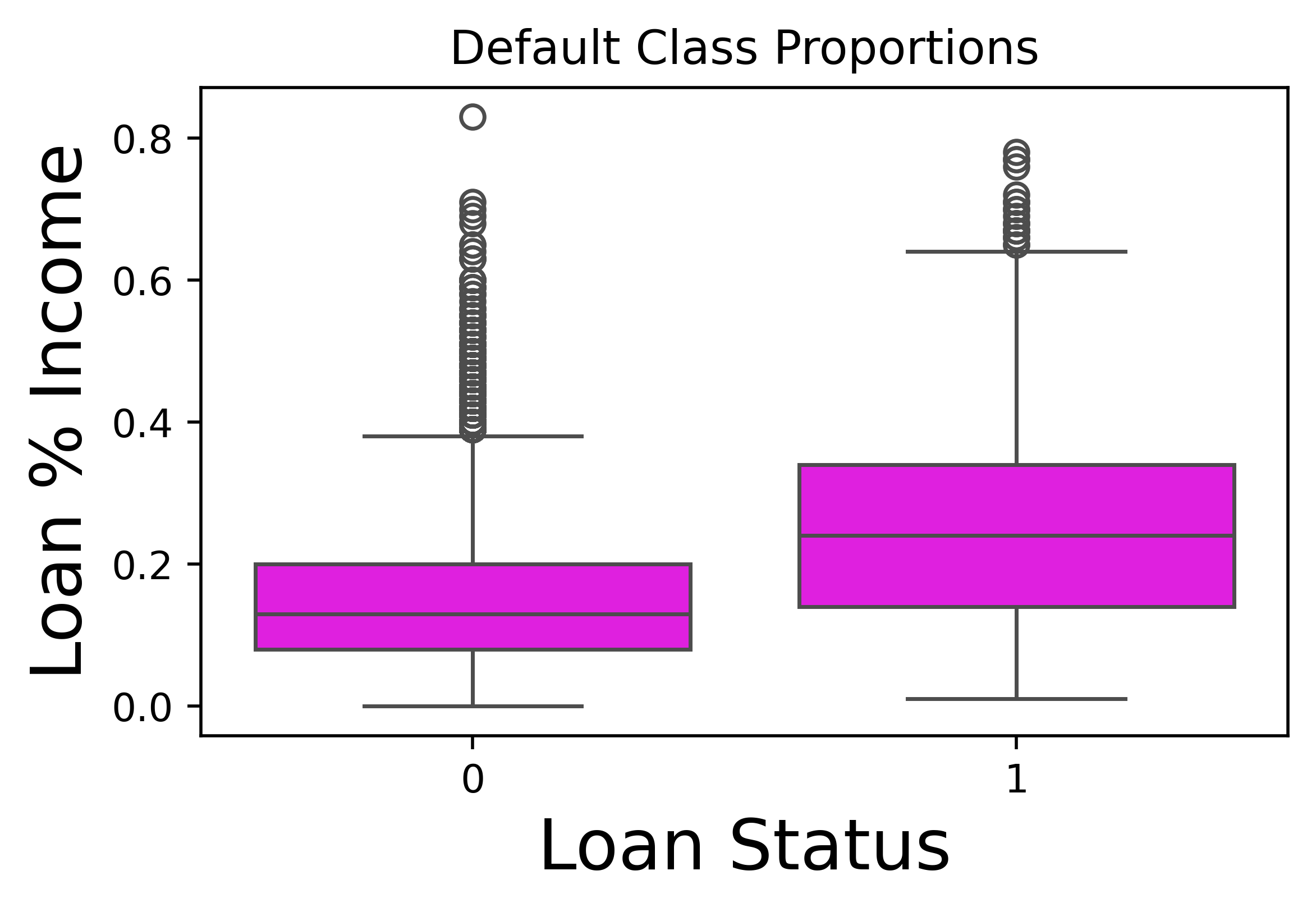
Relationship between loan-to-income ratio and default
One obvious pattern that can be anticipated is the fact that if a greater loan is taken against the income, the probability of default is higher. We can verify this as shown in the plot below.
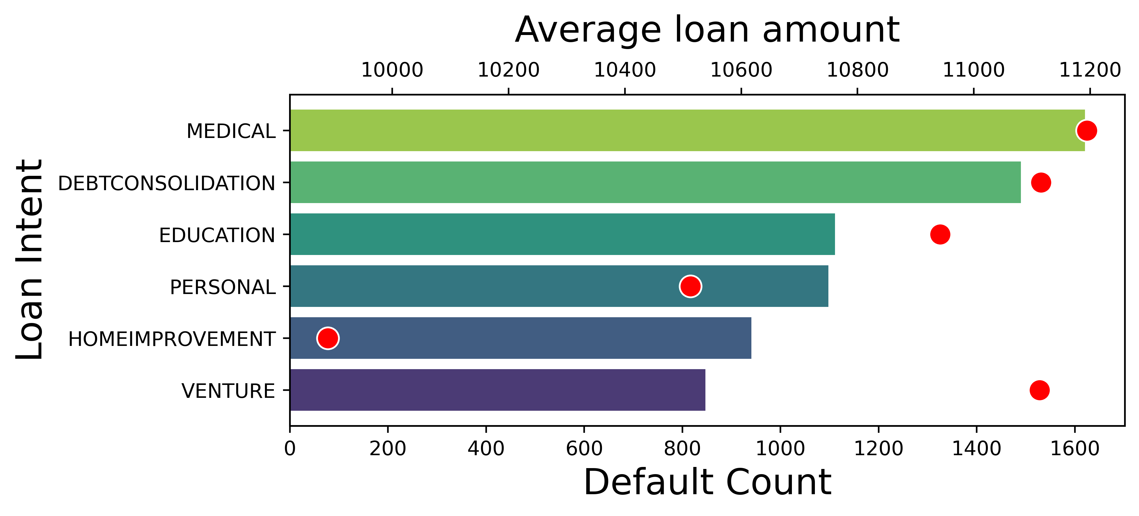
Data Exploration: Observing the sector-wise default cases
Understanding the number of default cases in each sector and the typical loan amount for such cases is quite interesting. For this, we use the pandas groupby library to create sector-wise groups and find the mean and count of each aggregate. I use pandas for this wrangling step since I will use it later to plot in Seaborn, which is available only in pandas, and it is much easier than using pyspark.
# extract out the cases where the default has occurred for different types of loans
default_cases = data_pds[data_pds['loan_status']==1]

# Compute the mean loan amount  and the size of all the default cases for each loan type
default_summary  = default_cases.groupby('loan_intent').agg({'loan_amnt':'mean', 'loan_status':'count'})
default_summary.columns = ['avg_loan_amount', 'default_count']

# sort values of most number of default cases
default_count = default_summary.sort_values(by = 'default_count', ascending = False)
print('sector with largest principle defaulted',default_summary)

# sort the average loan amount per intent type
avgloanamount = default_summary.sort_values(by= 'avg_loan_amount', ascending = False)
print('sector with most number of default cases', avgloanamount)
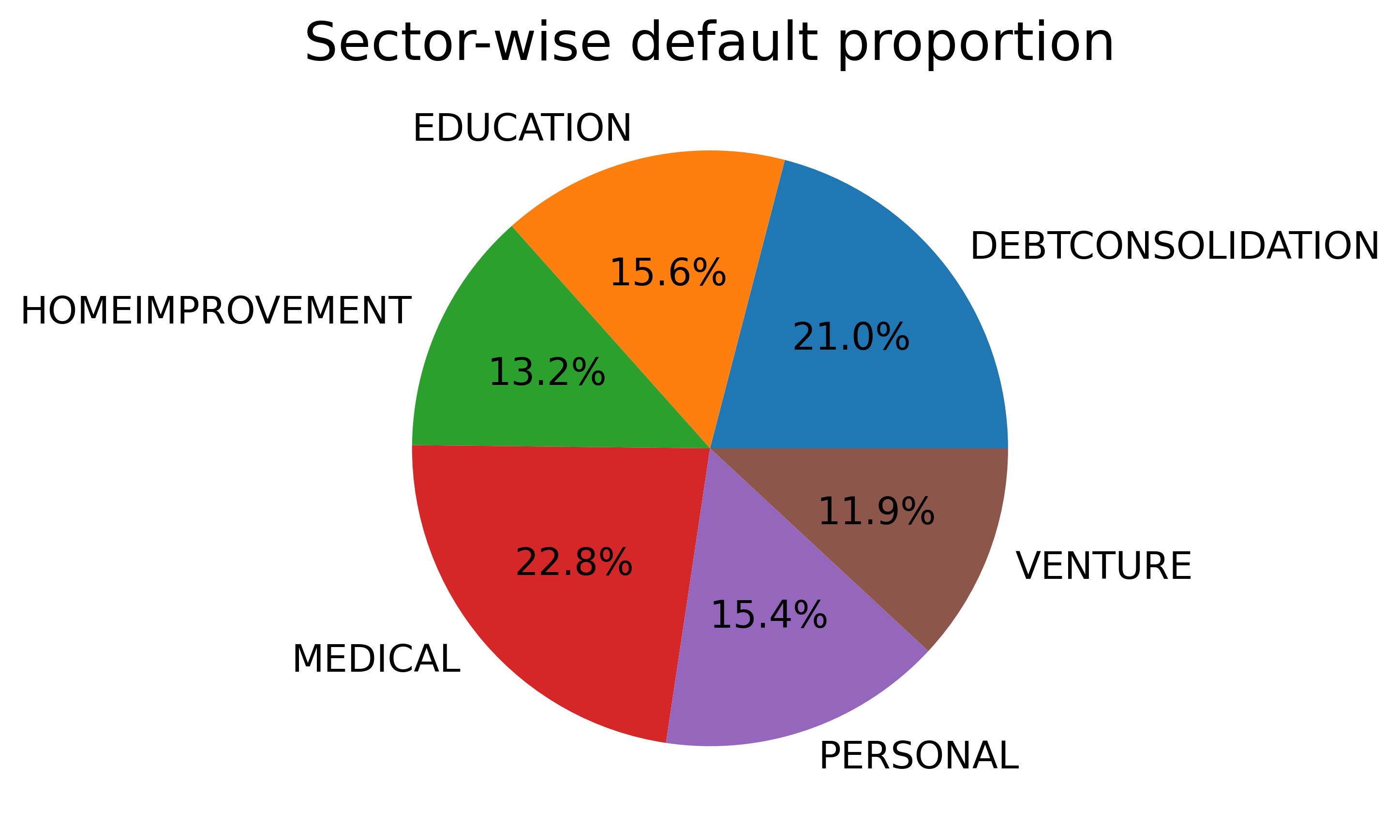
A better way to understand the count of the default cases is by making a pie chart, as shown below.
Predicting Defaults using Supervised Learning: Data Preprocessing
The most important step before performing any predictive analysis is to preprocess the data to prepare it for analysis. They can have several types of imperfections like: duplicates, missing values, unnormalised data columns, to name a few. Also, they might exist in a format that is difficult to use for predictive analysis, like non-numerical classes for categorical data. These elements are present in nearly all raw data; hence, nearly every raw dataset needs some form of transformation to increase its usability.
We shall use the following scheme to address the shortcomings in our current dataset:
1. Missing values shall be replaced with the median values since these parameters show a skewed distribution and have a significant amount of outliers.
2. We remove the means of each parameter and scale the variance to 1.
3. Convert the categorical data into numerical format using One-hot Encoding.
These pre-processing steps can be very easily implemented using the pipeline module of scikit-learn as shown below.
# Create the data sets and transform, normalise and split the data
X = data_pds[['person_age', 'person_income', 'person_emp_length', 'loan_amnt', 'loan_int_rate','person_home_ownership', 'loan_intent', 'cb_person_default_on_file']]
y = data_pds['loan_status']
X = X.drop(columns = ['loan_amnt'])

# The data that are in numbers format
numeric_features = ['person_age', 'person_income', 'person_emp_length', 'loan_int_rate']

# The data that is in the form of category
categorical_features = ['person_home_ownership', 'loan_intent', 'cb_person_default_on_file']

numerical_transformer = Pipeline(steps = [
('imputer', SimpleImputer(strategy = 'median')),
('scaler', StandardScaler())
])

categorical_transformer = Pipeline(steps = [
('imputer', SimpleImputer(strategy = 'most_frequent')),    # use the mode to replace the missing values
('onehot', OneHotEncoder(handle_unknown = 'ignore'))       # one-hot encoding
])

# create a preprocessing object with all the features in it...
preprocessor = ColumnTransformer(
transformers = [
('num', numerical_transformer, numeric_features),
('cat', categorical_transformer, categorical_features)
])

X_precessed = preprocessor.fit_transform(X)
categorical_columns  = preprocessor.transformers_[1][1]['onehot'].get_feature_names_out(categorical_features)
all_columns = numeric_features + list(categorical_columns)
Once the data is correctly preprocessed, we can split the data into a training and a testing set, setting a particular random state for consistency.
# split the data into train and test
X_train, X_test, y_train, y_test = train_test_split(X_precessed, y, test_size = 0.2, random_state = 42)
Model Training
For each ML technique, first an object is created, then fitted with the training data, and finally used on the test data to benchmark its predictive power. Then, we use the metrics module to map the accuracy, confusion matrix, and the classification report. The accuracy, as the name suggests, provides the predictive accuracy. The confusion matrix provides the class-wise performance, i.e., how much each class was correctly predicted and how much the model confused the prediction with the other class. It also indicates the precision and the recall of the prediction. The accuracy of the prediction is lost either in the form of precision or in the form of recall. Precision can be naively thought of as how precise the predictions are, whereas recall is how many of the actual cases were correctly identified.
Usually, there is a tradeoff between the precision and the recall. However, depending on the objective of the prediction, we can optimise this tradeoff. E.g., if we want to detect some critical illness, we would want the lowest possible recall. This means a large number of false positive cases might be reported. However, we can perform additional screening to subsequently remove these cases. Another example can be in the field of finance, where one would want to detect fraud. Low recall is needed to catch any fraud case.
I test four differernt 4 different techniques: Logistic regression, Random forests, K-Nearest neighbor classification, and Support Vector machines (SVM), which perform better on imbalanced datasets. I tested 3 different kernels of SVM, the linear, polynomial (n-3), and the RBF, commonly called the Gaussian kernel. Their implementation is shown in the code below
# testing logistic regression
logistic_classifier = LogisticRegression(random_state =42)
logistic_classifier.fit(X_train, y_train)

ypred = logistic_classifier.predict(X_test)

print('accuracy', accuracy_score(y_test, ypred))
print('confusion matrix', confusion_matrix(y_test, ypred))
print('classification report', classification_report(y_test, ypred))
# instantiate the random forest classifier
random_forest_classifier = RandomForestClassifier(random_state = 42)
random_forest_classifier.fit(X_train, y_train)
ypred = random_forest_classifier.predict(X_test)

print('accuracy', accuracy_score(y_test, ypred))
print('confusion matrix', confusion_matrix(y_test, ypred))
print('classification report', classification_report(y_test, ypred))

# instantiate and test the random forest classifier
knn_classifier = KNeighborsClassifier()
knn_classifier.fit(X_train, y_train)
ypred = knn_classifier.predict(X_test)

print('accuracy', accuracy_score(y_test, ypred))
print('confusion matrix', confusion_matrix(y_test, ypred))
print('classification report', classification_report(y_test, ypred))

# here we try the linear SVC
svm_clf = svm.LinearSVC() # linear kernal and 1:1 weights
svm_clf.fit(X_train, y_train)

ypred = svm_clf.predict(X_test)
print('accuracy', accuracy_score(y_test, ypred))
print('confusion matrix', confusion_matrix(y_test, ypred))
print('classification report', classification_report(y_test, ypred))

# here we try the poly SVC
svm_clf = svm.SVC(kernel= 'poly', degree = 3) # polynmomial kernal and 1:1 weights
svm_clf.fit(X_train, y_train)

ypred = svm_clf.predict(X_test)
print('accuracy', accuracy_score(y_test, ypred))
print('confusion matrix', confusion_matrix(y_test, ypred))
print('classification report', classification_report(y_test, ypred))

# here we try the rbf SVC
svm_clf = svm.SVC(kernel= 'rbf') # rbf and 1:1 weights
svm_clf.fit(X_train, y_train)

ypred = svm_clf.predict(X_test)
print('accuracy', accuracy_score(y_test, ypred))
print('confusion matrix', confusion_matrix(y_test, ypred))
print('classification report', classification_report(y_test, ypred))
Model Evaluation
Finally, we can tabulate the performance of each of these methods as follows:
| Model | Accuracy | Precision | Recall | F1 Score |
|---|---|---|---|---|
| Logistic Regression | 0.82 | 0.69 | 0.34 | 0.46 |
| Random Forest Classifier | 0.85 | 0.75 | 0.51 | 0.61 |
| Linear Support Vector Machine | 0.82 | 0.73 | 0.27 | 0.39 |
| Trinomial Support Vector Machine | 0.84 | 0.82 | 0.33 | 0.47 |
| Gaussian Support Vector Machine | 0.84 | 0.84 | 0.34 | 0.49 |
The Accuracy of all models is similar, with Random Forest classifier and non-linear SVMs performing better than the rest. The SVM with Gaussian kernel has the highest precision. For recall, again, Random Forest Classifier did the best and so is its F1 score. Overall, Random Forest performed better than all other models. However, I will take these metrics with a pinch of salt since nearly every model has a very poor F1 score for predicting default cases, and Random Forest performs decently. This is primarily due to the imbalance in the dataset and the best strategy would be to make the weights balanced while training the models.