Particle Tracking Velocimetry (PTV) using K-Nearest Neighbors (KNN)

For soft, condensed matter physics, tracking particulate matter flows is a cornerstone for understanding fluid behavior. Whether it understands fluid-solid interactions or whether it is for understanding the fluid flow itself: -- where the particles in the fluid act as tracers. Thus, if we suspend tiny, lightweight particles in any fluid and track their motion, we can infer the flow behavior of the fluid itself, even if the fluid is transparent … sounds cool right!!

If one has the liberty to dump a larger concentration of particles into the fluid, then the fluid flow redistributes the particles in different regions of the fluid based on their velocity. Thus, by cross-correlating the changes in positions of a bunch of these particles we can infer their speeds (for the curious ones.… this correlation process resembles convolution kernels a lot!!!.) This method is now popularly known as Particle Image Velocimetry (PIV).

PIV is extremely good for cases where the particles obediently follow the fluid flow without any active involvement. Thus, to measure the fluid flow, we can map the motion of an ensemble of these particles without the need for tracking individual particles.

Many a time, the particles are actively involved and modify the fluid dynamics through hydrodynamic perturbations. In such cases, measuring the motion of nearly every particle becomes very important. To do so, we use another very interesting technique called Particle Tracking Velocimetry (PTV). PTV is performed by taking multiple snapshots in quick succession of a moving particle and correlating their position across these multiple snapshots. So, how does this work??

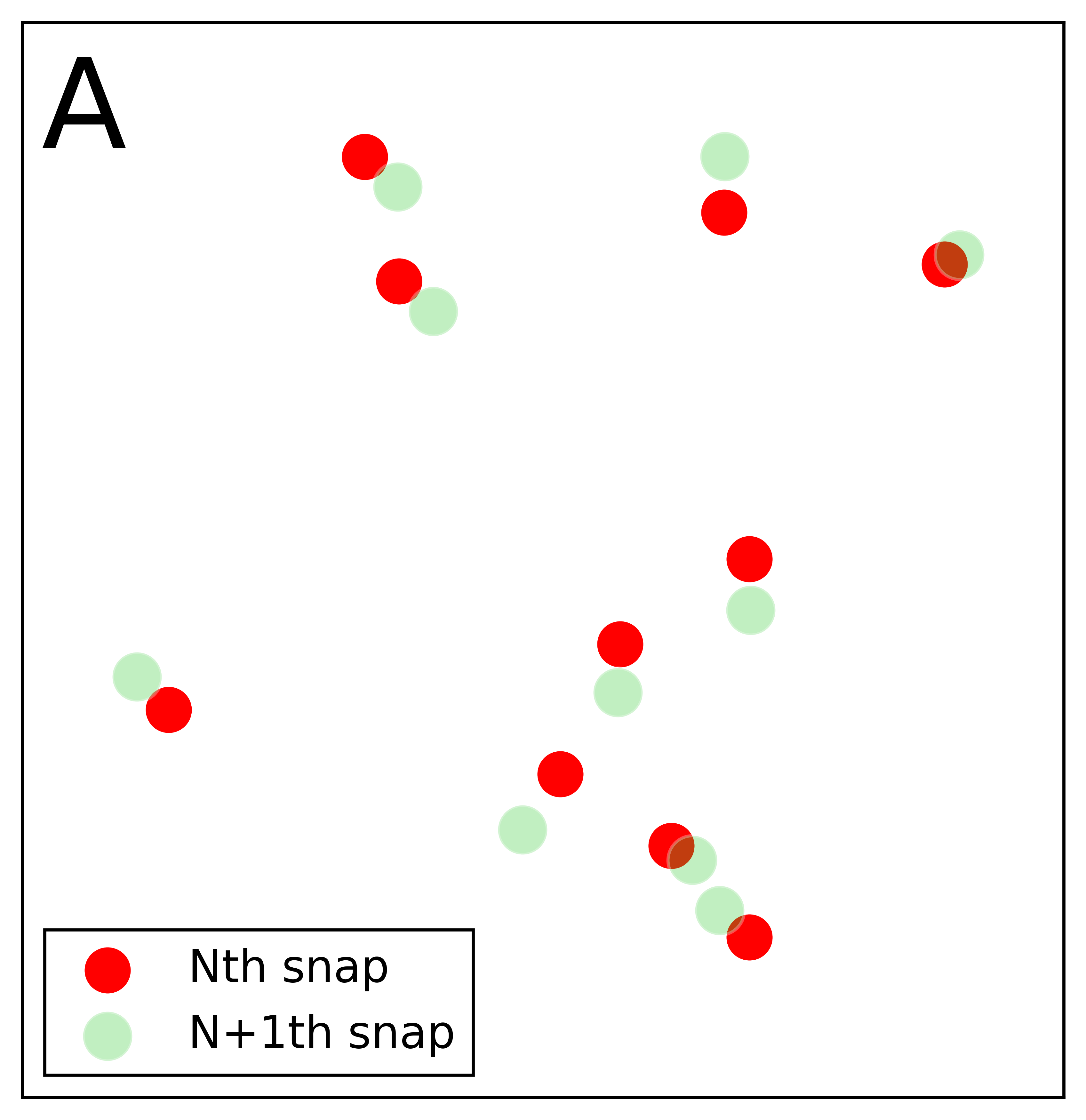
To understand this let's look at fig 1 which shows the superposition of two consecutive images of the particle. One can notice three interesting things

1. Between two successive snapshots, each particle drifts by a distance that corresponds to its speed at that instant. If the snaps are taken in quick succession, you can identify the image pairs for each particle by eye between the snaps.(see fig 1(a))
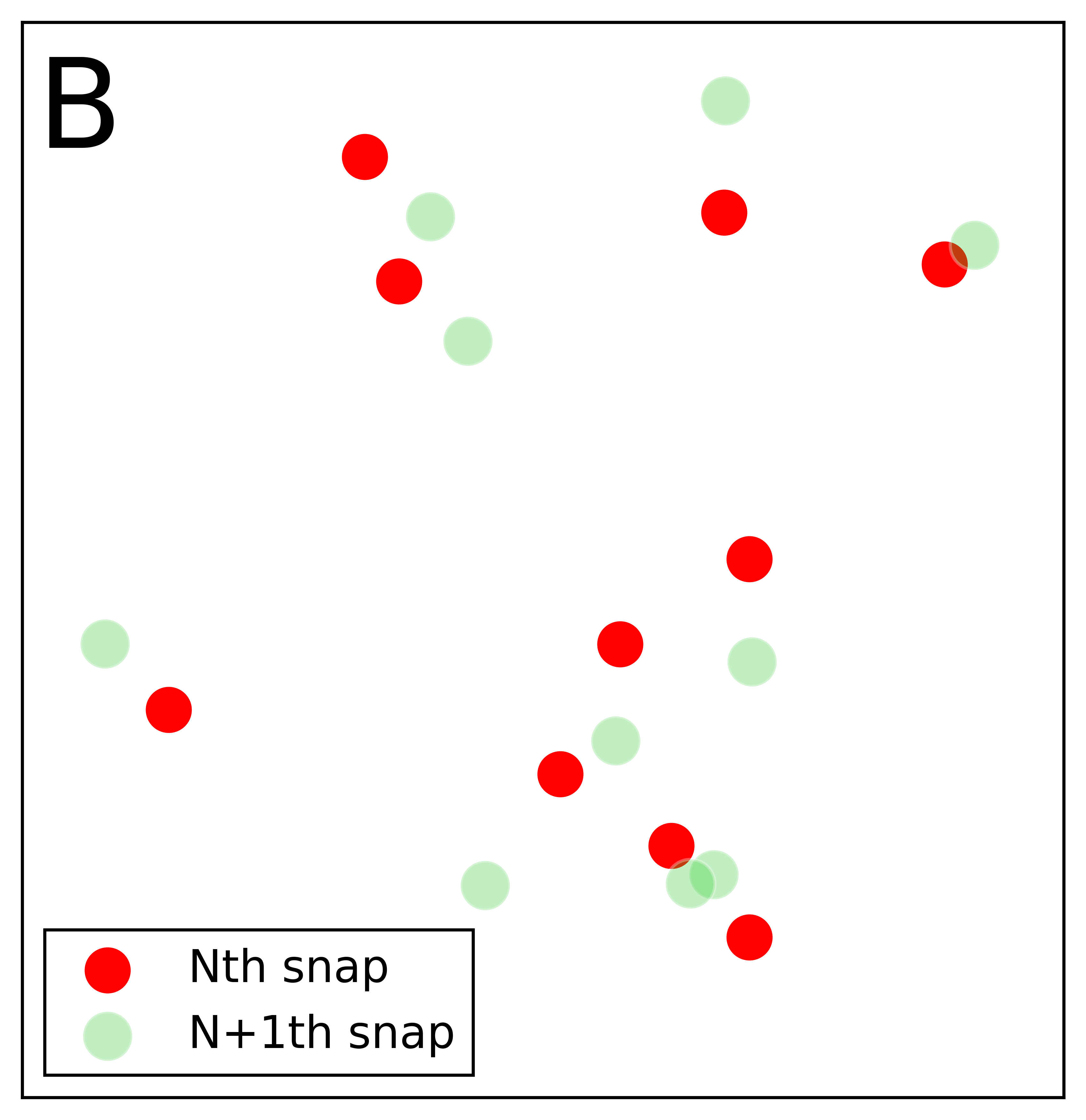
2. If the particle has traveled too far,(when there is a significant time delay in taking a snapshot) the position of the particle in the previous frame becomes difficult to trace by eye.(see fig 1(b))
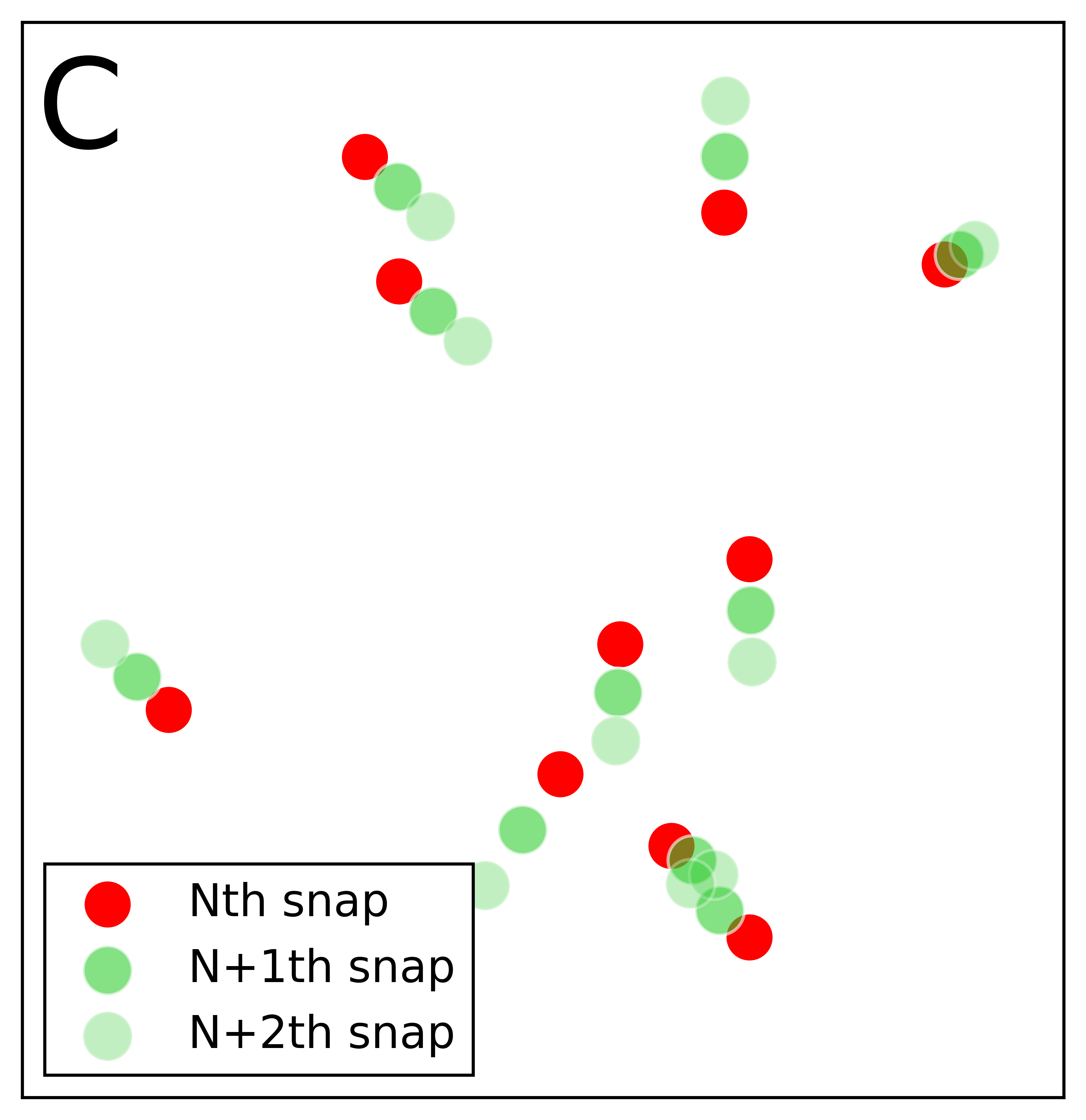
3. However, if we add an intermediate snapshot, it becomes fairly easy to trace.(see fig 1(c))

This is because our brain which is a beautiful neural network, searches for patterns to establish a single identity of a particle across several snapshots. This pattern is: finding the closest particle images between successive snapshots.
To do this, it estimates the distances of a particle’s image in a preceding snap to all particle images in the successive snap. Thus, ideally speaking, the nearest particle image in the successive snap will most likely be the image of itself!! (see fig 2). If the delay between two snaps is long, then the particles might have traveled far from their position in the preceding snapshot, enough to confuse our brains regarding the previous position of the particle. Hence we find it difficult to trace the original positions as in fig 1(b).

Most statisticians/data gurus/analysts/science nerds might have figured out by now how this trick can be mathematically implemented. Yes …… the answer is: using K Nearest Neighbors (KNN). Because the nearest neighbor (K=1) of any particle is its OWN IMAGE from the consecutive snapshot. So, what is KNN?

KNN is a technique by which we can search for the 'K' number of nearest neighbors of any entity. A simple example can be a classroom full of children where each child can use a measurement tape and measure out the nearest 3 classmates that are sitting around them. For this, it stands as K=3. KNN is one of the most versatile methods in statistics because balances perfectly between performance and simplicity. Also, it is flexible enough to be used for classification as well as regression problems.

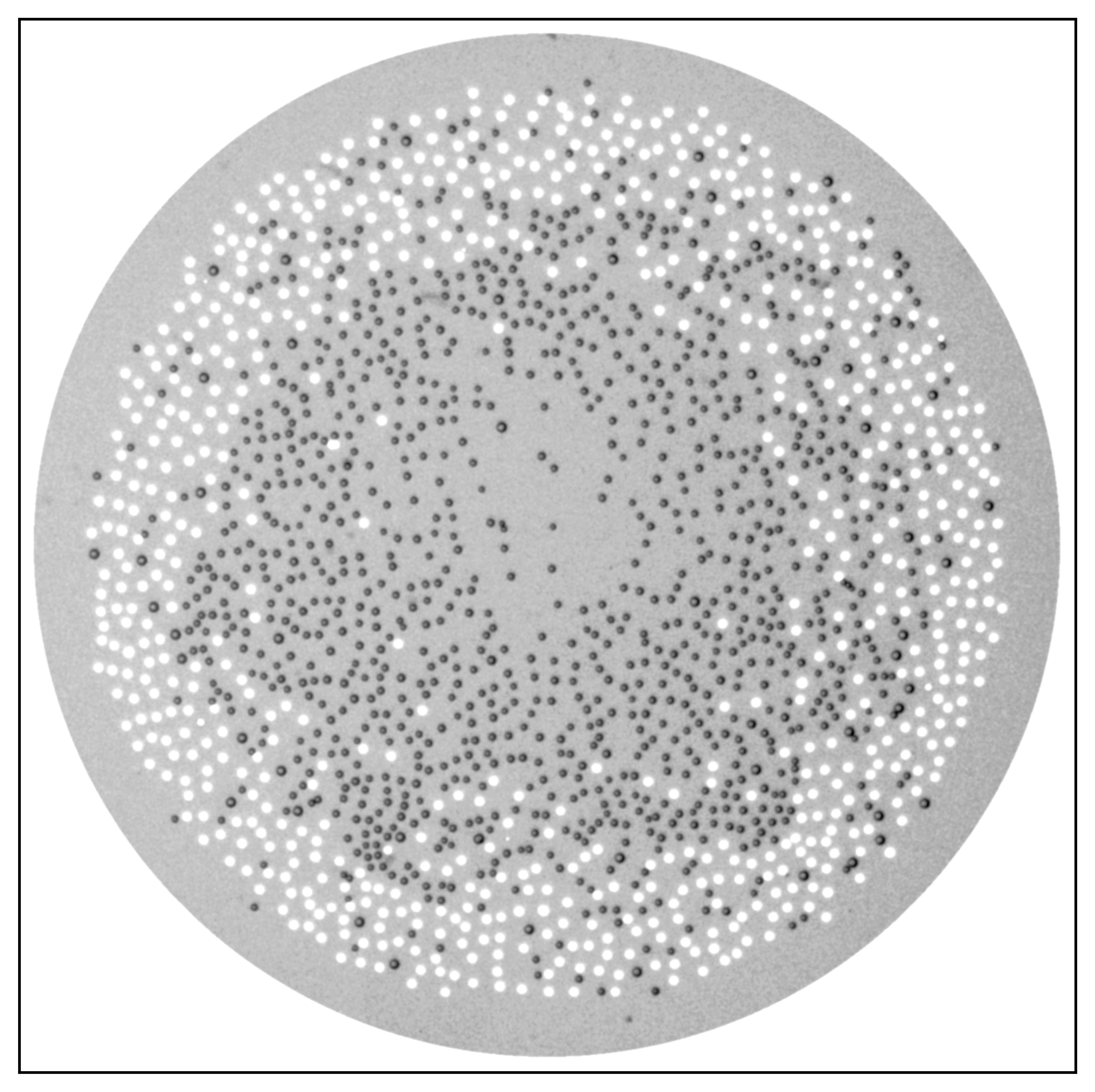
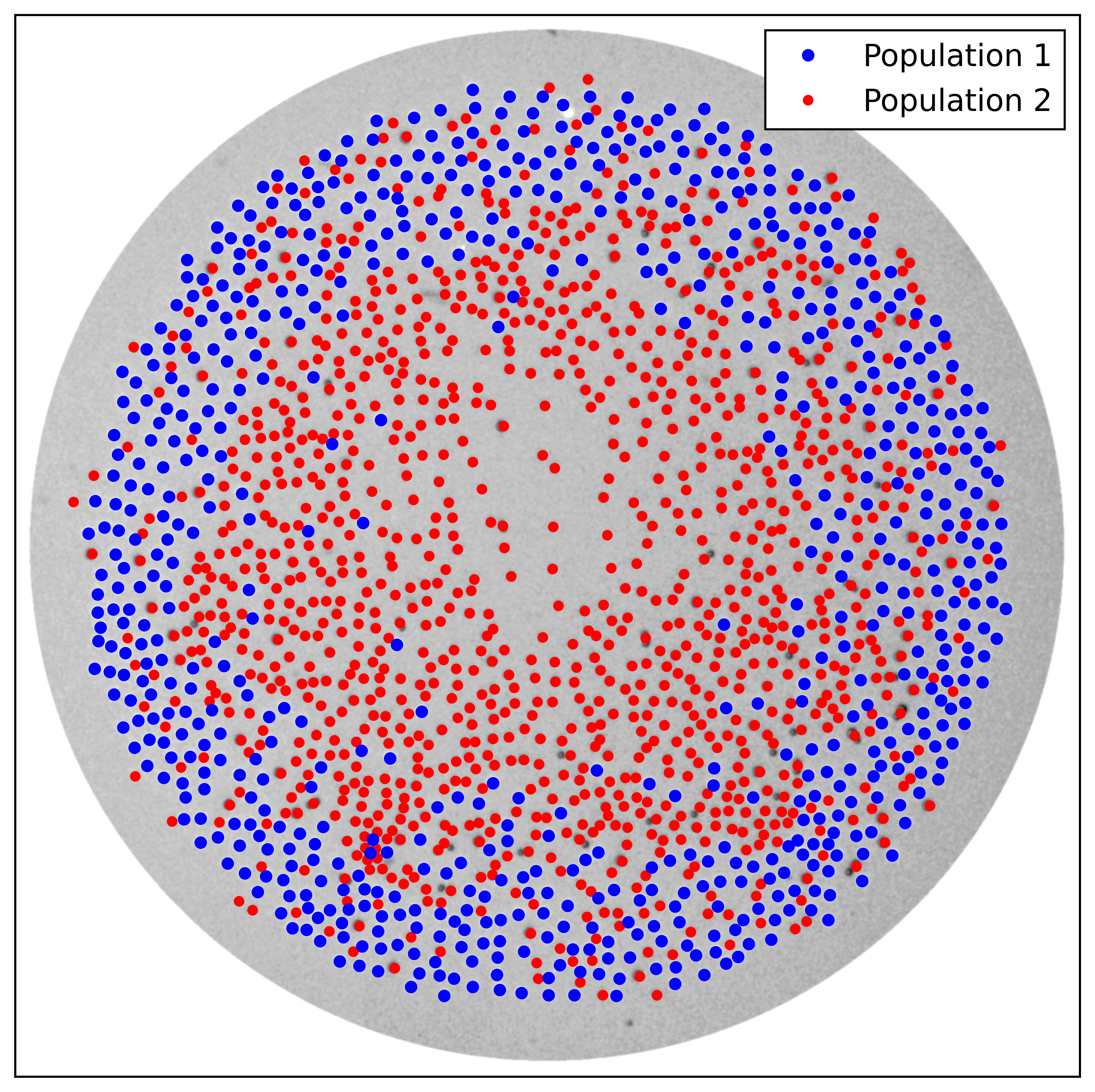
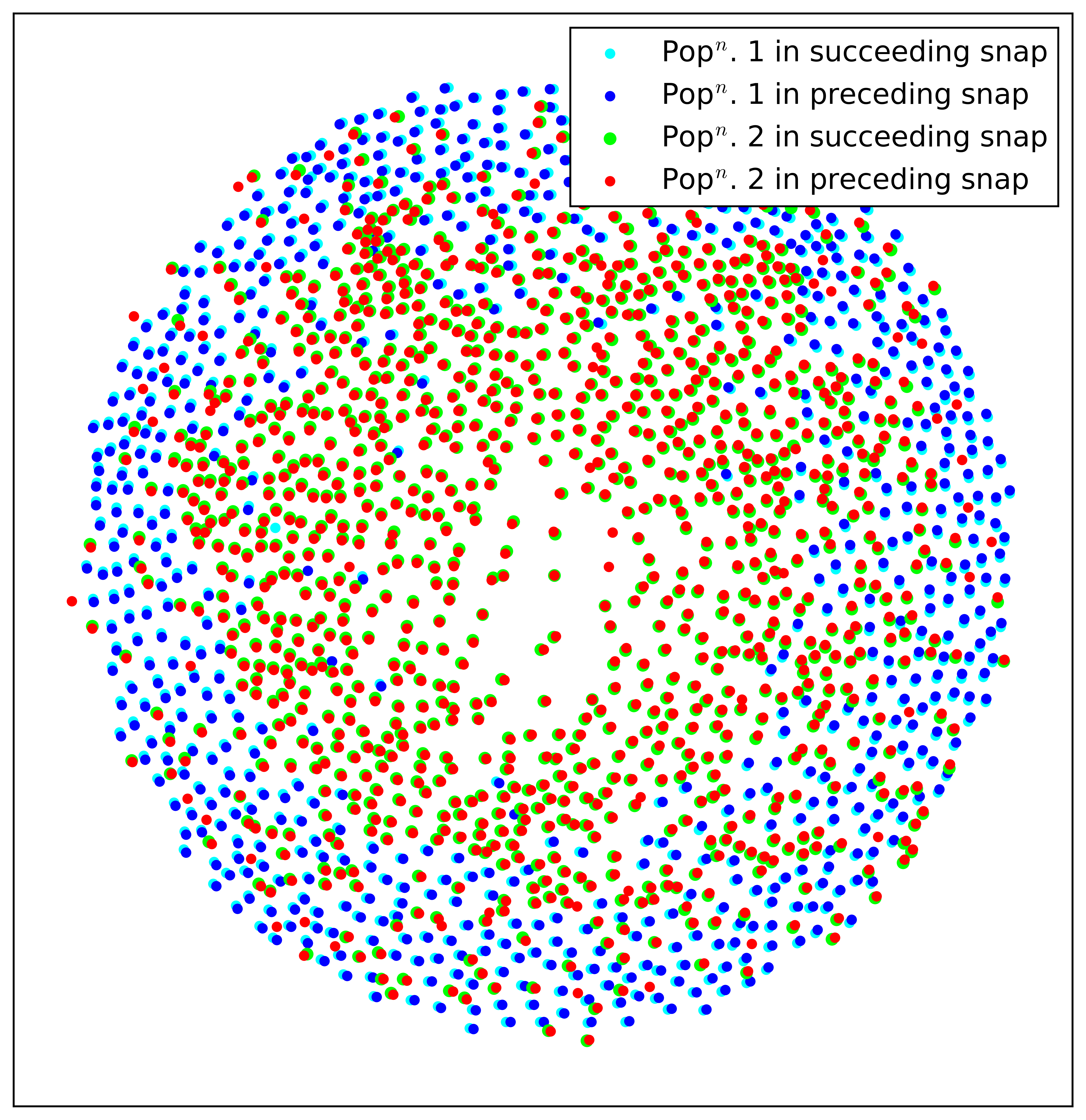
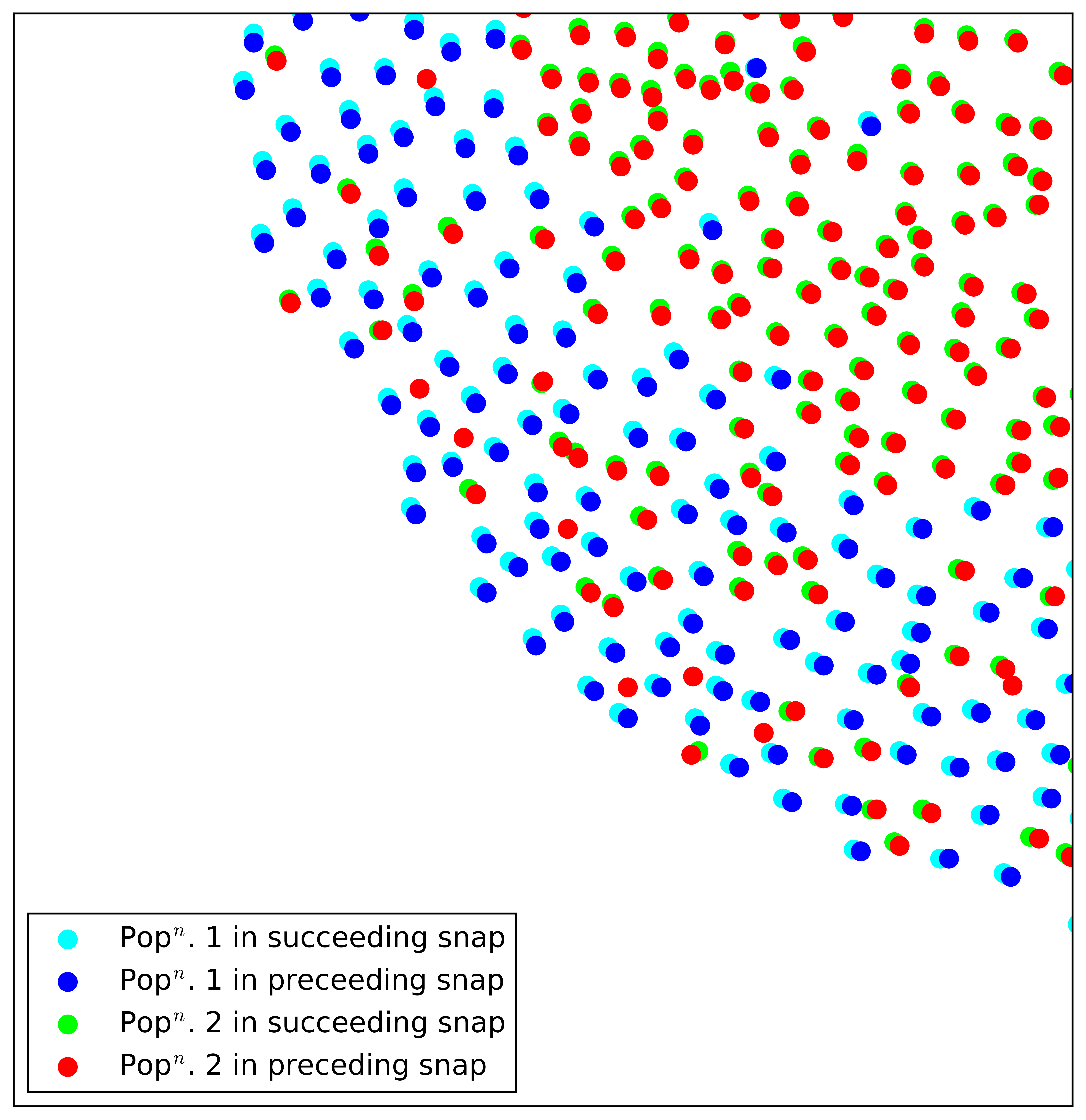
At this stage, I can demonstrate the power of KNN that drives PTV using a simple example from my PhD experiments. fig.3(a) shows a snapshot of two populations of particles moving inside a vortex. Using a computer vision software called ImageJ, I can identify each population pretty accurately, and I indicate them with red and blue colors as shown in fig 3(b). Now, I perform the same operation on the successive snapshot as well and overlay the coordinates on the previous snapshot as shown in fig. 4(a). You can appreciate how rapidly the subsequent snapshot was taken as the particles have moved very little, and this is visible more clearly in fig 4(b) where I zoom into the bottom left quadrant of the vortex. You can almost tell the image pairs for each particle just by looking at this figure!!

Now, to implement KNN mathematically, I define a function to search for the nearest neighbor (Visit my Github Repository to check out my Google Colab Notebook containing the code implementation. The simplest searching strategy is the ‘brute force’ method that first computes the distances between all possible image pairs. An image pair is created by picking 1 image from each frame. Then it chooses the ‘shortest’ distance. However, this is computationally very expensive (scales with a square of the number of particles), and there are better algorithms like ‘KD tree’ and ‘ball tree’ that use binary search to optimize the searching process(this scales linearly). I will discuss these algorithms in detail in some other post.

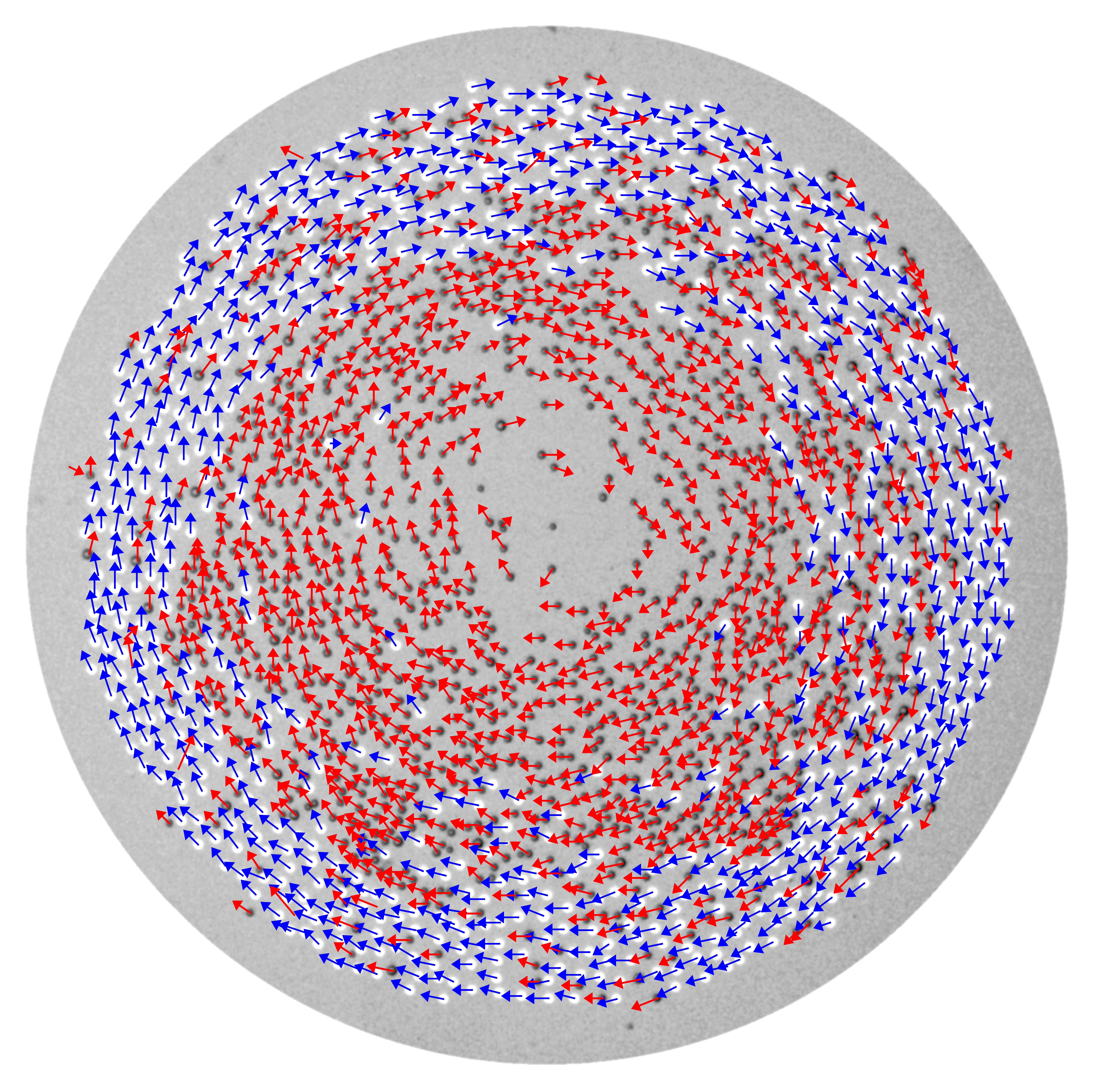
So, once the algorithm finds the image pair of each particle between the successive frames, it generates ‘indices’ as ‘tags’ which I then use to connect the correct image pair. Then I generate a ‘displacement’ vector, using the coordinates of the image pair. Unrealistic displacement vectors help me remove some wrongly connected image pairs (of course) that I ignore due to their statistical irrelevance. Fig 5 shows the final velocity vector computed from the displacement vectors simply by dividing it by the time lag between the two successive snapshots completing the PTV process between two snaps. Now, doing this between all snapshots of the experiment, I can trace the motion of nearly all particles throughout my entire experiment.

A definite question that comes to your mind by now: What snapshot rate is quick enough for successful and efficient particle tracking? Well, for real experiments, particles are finite-sized and occupy space, hence do not overlap. We exploit this to say that the imaging rate should be greater than D/V where D is the diameter of the particle and V is the speed of the fastest particle. Also, it should not be too quick: it should be slow enough for particle detection software (like imageJ) to detect a change in the particle position based on the camera’s image resolution.

Finally, I am sure you might now be curious to know about my experimental image and how the two populations of particles are beautifully segregated inside the ‘circular vortex’ ??? What is this vortex by the way??? and how are they even moving ???. All these answers are presented in my article published in the Physical Review Letters. You can watch the video in the research section of this website